Matrix in Ebitengine
This article explains what are matrices and how they are used in Ebitengine. We don't explain a strict mathematical theory. Instead, we explain essential knowledge for Ebitengine.
TL;DR
Ebitengine uses a mathematical matrix to specify how an image is transformed geometrically like scaling or rotating. A combination of multiple geometric transforms can be represented by one matrix.
Coordinate System
Ebitengine treats 2D graphics, and defines its coordinate system. X axis is rightward, and Y axis is downward. The origin point is upper left.
The coordinate system exists for each ebiten.Image object. The upper left point of the destination image is the origin point of the coordinate system.

Matrix
ebiten.Image is a set of pixels on a 2D rectangle. In Ebitengine, you can apply a conversion rule for each pixel. By the conversion rule, you can put an image at a specified position, and you can also apply various effects like scaling or rotating. As a conversion rule, Ebitengine uses a matrix.
In 2D space, a point is represented as a 2D vector (x, y). A 2D matrix converts this and generates a new point.

Definition
A matrix is a mathematical value used in linear algebra. A matrix is an array of numbers. A 2D matrix is like this.
\begin{aligned} \begin{bmatrix} 0.5000 & -0.8660 \\ 0.8660 & 0.5000 \\ \end{bmatrix} \end{aligned}
The horizontal sequences are called rows, and the vertical sequences are called columns. If the size is 2, the matrix is called 2D (two-dimensional) matrix, and if 3, 3D (three-dimensional) matrrix. A 3D matrix is like this.
\begin{aligned} \begin{bmatrix} 0.2990 & 0.5870 & 0.1140 \\ -0.1687 & -0.3313 & 0.5000 \\ 0.5000 & -0.4187 & -0.0813 \\ \end{bmatrix} \end{aligned}
If the numbers of columns and rows are the same, the matrix is called a regular matrix. Ebitengine treats only regular matrices.
Multiplying a matrix and a vector
You can multiply a matrix and a vector. The matrix is on the left side and the vector is on the right side. In general mathematics, the swapped positions are also possible but Ebitengine doesn't treat the swapped positions.
A matrix is a conversion rule, and in the equation, (x, y) means a point before converting, multiplying means applying the conversion rule, and (ax+by, cx+dy) means a point after converting.
\begin{aligned} \begin{bmatrix} a & b \\ c & d \\ \end{bmatrix} \begin{bmatrix} x \\ y \\ \end{bmatrix} = \begin{bmatrix} ax + by \\ cx + dy \\ \end{bmatrix} \end{aligned}
By the way, this is the same in the three-dimensional case.
\begin{aligned} \begin{bmatrix} a & b & c \\ d & e & f \\ g & h & i \\ \end{bmatrix} \begin{bmatrix} x \\ y \\ z \\ \end{bmatrix} = \begin{bmatrix} ax + by + cz \\ dx + ey + fz \\ gx + hy + iz \\ \end{bmatrix} \end{aligned}
Identity matrix
An identity matrix is a matrix that doesn't change the multiplicand.
\begin{aligned} \begin{bmatrix} 1 & 0 \\ 0 & 1 \\ \end{bmatrix} \end{aligned}
Let's multiply this identity matrix and a vector. You can confirm that the input and the output are the same. This matrix doesn't change any points on a 2D space.
\begin{aligned} \begin{bmatrix} 1 & 0 \\ 0 & 1 \\ \end{bmatrix} \begin{bmatrix} x \\ y \\ \end{bmatrix} = \begin{bmatrix} 1 \cdot x + 0 \cdot y \\ 0 \cdot y + 1 \cdot y \\ \end{bmatrix} = \begin{bmatrix} x \\ y \\ \end{bmatrix} \end{aligned}
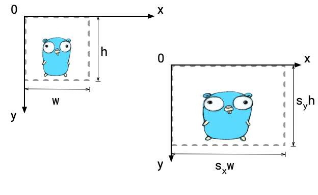
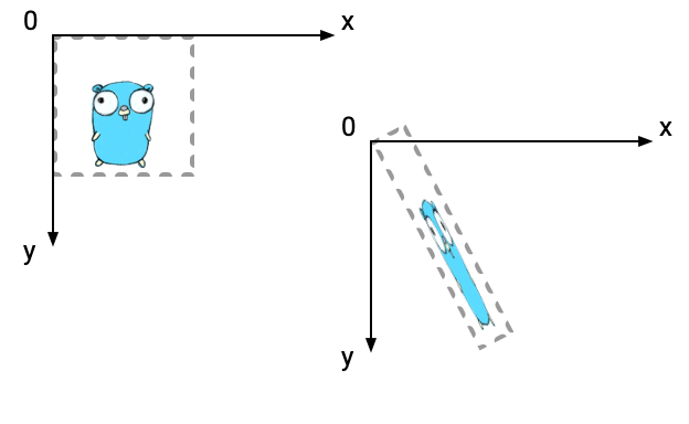
Scaling
A matrix that scales an image by s_x times in X direction and by s_y times in Y direction centering at the origin is this.
\begin{aligned} \begin{bmatrix} s_x & 0 \\ 0 & s_y \\ \end{bmatrix} \end{aligned}
Let's multiply this matrix and a vector.
\begin{aligned} \begin{bmatrix} s_x & 0 \\ 0 & s_y \\ \end{bmatrix} \begin{bmatrix} x \\ y \\ \end{bmatrix} = \begin{bmatrix} s_x \cdot x + 0 \cdot y \\ 0 \cdot x + s_y \cdot y \\ \end{bmatrix} = \begin{bmatrix} s_x x \\ s_y y \\ \end{bmatrix} \end{aligned}
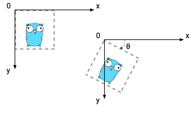
Rotating
A matrix that rotates an image by an angle \theta centering at the origin is this. This uses trigonometric functions. Please don't worry if you don't know trigonometric functions. Ebitengine has a useful function to rotate images.
\begin{aligned} \begin{bmatrix} \cos \theta & -\sin \theta \\ \sin \theta & \cos \theta \\ \end{bmatrix} \end{aligned}
Multiplying a matrix and a matrix
For example, what if you want to combine scaling and rotating? To come to the point, such combinations of conversion rules can be represented as one matrix. Let's see how two matrices are combined.
If a vector is multiplied by two matrices, the equation will be like this.
\begin{aligned} \begin{bmatrix} a_2 & b_2 \\ c_2 & d_2 \\ \end{bmatrix} \begin{bmatrix} a_1 & b_1 \\ c_1 & d_1 \\ \end{bmatrix} \begin{bmatrix} x \\ y \\ \end{bmatrix} &= \begin{bmatrix} a_2 & b_2 \\ c_2 & d_2 \\ \end{bmatrix} \begin{bmatrix} a_1 x + b_1 y \\ c_1 x + d_1 y \\ \end{bmatrix} \\ &= \begin{bmatrix} a_2(a_1 x + b_1 y) + b_2(c_1 x + d_1 y) \\ c_2(a_1 x + b_1 y) + d_2(c_1 x + d_1 y) \\ \end{bmatrix} \\ &= \begin{bmatrix} a_2 a_1 x + a_2 b_1 y + b_2 c_1 x + b_2 d_1 y \\ c_2 a_1 x + a_2 b_1 y + d_2 c_1 x + d_2 d_1 y \\ \end{bmatrix} \\ &= \begin{bmatrix} a_2 a_1 x + b_2 c_1 x + a_2 b_1 y + b_2 d_1 y \\ c_2 a_1 x + d_2 c_1 x + a_2 b_1 y + d_2 d_1 y \\ \end{bmatrix} \\ &= \begin{bmatrix} (a_2 a_1 + b_2 c_1) x + (a_2 b_1 + b_2 d_1) y \\ (c_2 a_1 + d_2 c_1) x + (c_2 b_1 + d_2 d_1) y \\ \end{bmatrix} \\ &= \begin{bmatrix} a_2 a_1 + b_2 c_1 & a_2 b_1 + b_2 d_1 \\ c_2 a_1 + d_2 c_1 & c_2 b_1 + d_2 d_1 \\ \end{bmatrix} \begin{bmatrix} x \\ y \\ \end{bmatrix} \end{aligned}
What an intimidating equation! However, this is a very beautiful result. This equation means that we can define multiplying two matrices like this.
\begin{aligned} \begin{bmatrix} a_2 & b_2 \\ c_2 & d_2 \\ \end{bmatrix} \begin{bmatrix} a_1 & b_1 \\ c_1 & d_1 \\ \end{bmatrix} = \begin{bmatrix} a_2 a_1 + b_2 c_1 & a_2 b_1 + b_2 d_1 \\ c_2 a_1 + d_2 c_1 & c_2 b_1 + d_2 d_1 \\ \end{bmatrix} \end{aligned}
Then, we were able to define the combination of two conversions as another matrix.
You don't have to remember this equation, but please remember the fact that multiplying two matrices results in one matrix.
By the way, in three-dimensional cases, multiplying will be like this.
\begin{aligned} & \begin{bmatrix} a_2 & b_2 & c_2 \\ d_2 & e_2 & f_2 \\ g_2 & h_2 & i_2 \\ \end{bmatrix} \begin{bmatrix} a_1 & b_1 & c_1 \\ d_1 & e_1 & f_1 \\ g_1 & h_1 & i_1 \\ \end{bmatrix} \\ =& \begin{bmatrix} a_2 a_1 + b_2 d_1 + c_2 d_1 & a_2 b_1 + b_2 e_1 + c_2 h_1 & a_2 c_1 + b_2 f_1 + c_2 i_1 \\ d_2 a_1 + e_2 d_1 + f_2 d_1 & d_2 b_1 + e_2 e_1 + f_2 h_1 & d_2 c_1 + e_2 f_1 + f_2 i_1 \\ g_2 a_1 + h_2 d_1 + i_2 d_1 & g_2 b_1 + h_2 e_1 + i_2 h_1 & g_2 c_1 + h_2 f_1 + i_2 i_1 \\ \end{bmatrix} \end{aligned}
Be careful that the order of multiplying matters. If there is a matrix A and a matrix B, the results of AB and BA are different in general. For example, \big[\begin{smallmatrix}1&2\\3&4\end{smallmatrix}\big]\big[\begin{smallmatrix}5&6\\7&8\end{smallmatrix}\big] is different from \big[\begin{smallmatrix}5&6\\7&8\end{smallmatrix}\big]\big[\begin{smallmatrix}1&2\\3&4\end{smallmatrix}\big]. In the context of conversion rule, rotating and scaling an image in this order is different from scaling and rotating the image in this order in general.
\begin{aligned} \begin{bmatrix} 1 & 2 \\ 3 & 4 \\ \end{bmatrix} \begin{bmatrix} 5 & 6 \\ 7 & 8 \\ \end{bmatrix} &= \begin{bmatrix} 19 & 22 \\ 43 & 50 \\ \end{bmatrix} \\ \begin{bmatrix} 5 & 6 \\ 7 & 8 \\ \end{bmatrix} \begin{bmatrix} 1 & 2 \\ 3 & 4 \\ \end{bmatrix} &= \begin{bmatrix} 23 & 34 \\ 31 & 46 \\ \end{bmatrix} \\ \begin{bmatrix} 1 & 2 \\ 3 & 4 \\ \end{bmatrix} \begin{bmatrix} 5 & 6 \\ 7 & 8 \\ \end{bmatrix} &\ne \begin{bmatrix} 5 & 6 \\ 7 & 8 \\ \end{bmatrix} \begin{bmatrix} 1 & 2 \\ 3 & 4 \\ \end{bmatrix} \end{aligned}
Affine transformation
A 2D matrix looks enough to move points, but there is a problem. Any 2D matrices cannot move the origin point (0, 0).
\begin{aligned} \begin{bmatrix} a & b \\ c & d \\ \end{bmatrix} \begin{bmatrix} 0 \\ 0 \\ \end{bmatrix} = \begin{bmatrix} a \cdot 0 & b \cdot 0 \\ c \cdot 0 & d \cdot 0 \\ \end{bmatrix} = \begin{bmatrix} 0 \\ 0 \\ \end{bmatrix} \end{aligned}
So can't we represent translating by matrices?
Then, we introduce an affine transform matrix. For 2D vectors, an affine transform matrix is like this. The matrix is extended to be three-dimensional. The last row is always (0, 0, 1).
\begin{aligned} \begin{bmatrix} a & b & t_x \\ c & d & t_y \\ 0 & 0 & 1 \\ \end{bmatrix} \end{aligned}
The vector will also be extended to three dimensional, and the third value is always 1. A 2D vector (x, y) will be (x, y, 1).
\begin{aligned} \begin{bmatrix} x \\ y \\ 1 \\ \end{bmatrix} \end{aligned}
Let's multiply this affine transform matrix and the extended vector. You can confirm that the result includes new terms t_x and t_y.
\begin{aligned} \begin{bmatrix} a & b & t_x \\ c & d & t_y \\ 0 & 0 & 1 \\ \end{bmatrix} \begin{bmatrix} x \\ y \\ 1 \\ \end{bmatrix} = \begin{bmatrix} a \cdot x + b \cdot y + t_x \cdot 1 \\ c \cdot x + d \cdot y + t_y \cdot 1 \\ 0 \cdot x + 0 \cdot y + 1 \cdot 1 \\ \end{bmatrix} = \begin{bmatrix} ax + by + t_x \\ cx + dy + t_y \\ 1 \\ \end{bmatrix} \end{aligned}
Translating
A matrix that just translates an image is this.
\begin{aligned} \begin{bmatrix} 1 & 0 & t_x \\ 0 & 1 & t_y \\ 0 & 0 & 1 \\ \end{bmatrix} \end{aligned}
Let's apply this matrix to a vector (x, y, 1). The result is translating x and y by t_x and t_y respectively.
\begin{aligned} \begin{bmatrix} 1 & 0 & t_x \\ 0 & 1 & t_y \\ 0 & 0 & 1 \\ \end{bmatrix} \begin{bmatrix} x \\ y \\ 1 \\ \end{bmatrix} = \begin{bmatrix} 1 \cdot x + 0 \cdot y + t_x \cdot 1 \\ 0 \cdot x + 1 \cdot y + t_y \cdot 1 \\ 0 \cdot x + 0 \cdot y + 1 \cdot 1 \\ \end{bmatrix} = \begin{bmatrix} x + t_x \\ y + t_y \\ 1 \\ \end{bmatrix} \end{aligned}
![]()
Scaling and rotating matrix we already explained will be a matrix that t_x and t_y are 0.
We don't prove this here, but multiplying two affine transform matrices results in an affine transform matrix. This means that any combinations of scaling, rotating and translating are represented as one affine transform matrix. Based on this fact, Ebitengine's API for geometric transform is very simple and requires only one affine transform matrix. Ebitengine's matrices are always affine transform, and doesn't treat other matrices.
Filter
We explained that converting an image is represented by a matrix that moves each pixel of the image. You might already realize this, but as a matter of fact, enlarging an image in this way results in an image with full of holes, since the destination area is larger than the source area. To avoid such odd results, Ebitengine complements pixels by filters. The way in which the pixels are complemented is determined by a filter type, like ebiten.FilterNearest or ebiten.FilterLinear
Color matrix
In Ebitengine, matrices are also used when converting colors. We don't explain details here. Ebitengine treats an RGBA color as a point in 4D space, and convert it with a matrix. The matrix is an affine transform matrix, and the dimension is 5.
\begin{aligned} \begin{bmatrix} x_1 & x_2 & x_3 & x_4 & t_r \\ x_5 & x_6 & x_7 & x_8 & t_g \\ x_9 & x_{10} & x_{11} & x_{12} & t_b \\ x_{13} & x_{14} & x_{15} & x_{16} & t_a \\ 0 & 0 & 0 & 0 & 1 \\ \end{bmatrix} \begin{bmatrix} r \\ g \\ b \\ a \\ 1 \\ \end{bmatrix} \end{aligned}
References
Ebitengine における行列
この記事では、 行列とは何か、行列を Ebitengine でどう使うのかについて説明します。厳密な数学の理論は説明しません。代わりに、 Ebitengine のためのエッセンスを紹介します。
要約
Ebitengine は数学の「行列」を、画像の拡大縮小や回転などの変換指定に用います。複数の幾何変換行列の組み合わせは、 1 つの行列で表されます。
座標系
Ebitengine は 2 次元のグラフィックスを扱い、その座標系を定めています。 X 軸は右方向で、 Y 軸は下方向です。原点は左上です。
座標系は各 ebiten.Image ごとに存在します。描画先画像の左上の点が座標系の原点になります。
行列
ebiten.Image は 2 次元矩形のピクセルの集合です。 Ebitengine では、各ピクセルに変換ルールを施すことができます。この変換ルールによって、画像を指定した位置に描画したり、また拡大縮小や回転などの様々なエフェクトを施すことが出来ます。変換ルールとして、 Ebitengine は行列を使用します。
2 次元空間上では、点は 2 次元ベクトル (x, y) で表されます。 2 次元行列はこれを変換し、新しい点を生成します。
定義
行列は線形代数で使われる数学的な値です。行列は数字の配列です。 2 次行列は次のようなものです:
\begin{aligned} \begin{bmatrix} 0.5000 & -0.8660 \\ 0.8660 & 0.5000 \\ \end{bmatrix} \end{aligned}
水平な並びは行、垂直な並びは列と呼ばれます。大きさが 2 ならば、行列は 2 次行列と呼ばれ、また 3 ならば 3 次行列と呼ばれます。 3 次行列は次のようなものです:
\begin{aligned} \begin{bmatrix} 0.2990 & 0.5870 & 0.1140 \\ -0.1687 & -0.3313 & 0.5000 \\ 0.5000 & -0.4187 & -0.0813 \\ \end{bmatrix} \end{aligned}
行と列の数が同じならば、その行列は正方行列と呼ばれます。 Ebitengine は正方行列のみ取り扱います。
行列とベクトルの乗算
行列とベクトルを掛け算することが出来ます。行列は左側、ベクトルは右側です。一般的な数学では、逆の位置もありえますが、 Ebitengine は逆の位置は取り扱いません。
行列は変換ルールであり、次の等式では (x, y) は変換前の点、乗算は変換ルールの適用、 (ax+by, cx+dy) は変換後の点を表しています。
\begin{aligned} \begin{bmatrix} a & b \\ c & d \\ \end{bmatrix} \begin{bmatrix} x \\ y \\ \end{bmatrix} = \begin{bmatrix} ax + by \\ cx + dy \\ \end{bmatrix} \end{aligned}
ところで、これは 3 次の場合でも同じです。
\begin{aligned} \begin{bmatrix} a & b & c \\ d & e & f \\ g & h & i \\ \end{bmatrix} \begin{bmatrix} x \\ y \\ z \\ \end{bmatrix} = \begin{bmatrix} ax + by + cz \\ dx + ey + fz \\ gx + hy + iz \\ \end{bmatrix} \end{aligned}
単位行列
単位行列は、掛けられる側を何も変えない行列です。
\begin{aligned} \begin{bmatrix} 1 & 0 \\ 0 & 1 \\ \end{bmatrix} \end{aligned}
単位行列とベクトルを掛け算してみましょう。
\begin{aligned} \begin{bmatrix} 1 & 0 \\ 0 & 1 \\ \end{bmatrix} \begin{bmatrix} x \\ y \\ \end{bmatrix} = \begin{bmatrix} 1 \cdot x + 0 \cdot y \\ 0 \cdot y + 1 \cdot y \\ \end{bmatrix} = \begin{bmatrix} x \\ y \\ \end{bmatrix} \end{aligned}
拡大
画像を X 軸方向に s_x、 Y 軸方向に s_y だけ、原点中心に拡大させるような行列は次のようなものです:
\begin{aligned} \begin{bmatrix} s_x & 0 \\ 0 & s_y \\ \end{bmatrix} \end{aligned}
行列とベクトルを掛け算してみましょう。
\begin{aligned} \begin{bmatrix} s_x & 0 \\ 0 & s_y \\ \end{bmatrix} \begin{bmatrix} x \\ y \\ \end{bmatrix} = \begin{bmatrix} s_x \cdot x + 0 \cdot y \\ 0 \cdot x + s_y \cdot y \\ \end{bmatrix} = \begin{bmatrix} s_x x \\ s_y y \\ \end{bmatrix} \end{aligned}
回転
画像を \theta の角度だけ、原点中心に回転させるような行列は次のようになります。これは三角関数を使用しています。三角関数について知らなくても大丈夫です。 Ebitengine には、画像を回転させる便利な関数があります。
\begin{aligned} \begin{bmatrix} \cos \theta & -\sin \theta \\ \sin \theta & \cos \theta \\ \end{bmatrix} \end{aligned}
行列と行列の乗算
例えば、拡大と回転を組み合わせたい場合はどうしたら良いでしょうか? 単刀直入に言うと、そのような変換ルールも 1 つの行列として表されます。どのように 2 つの行列を組み合わせるのか見てみましょう。
もしベクトルに 2 つの行列を掛けると、等式は次のようになります。
\begin{aligned} \begin{bmatrix} a_2 & b_2 \\ c_2 & d_2 \\ \end{bmatrix} \begin{bmatrix} a_1 & b_1 \\ c_1 & d_1 \\ \end{bmatrix} \begin{bmatrix} x \\ y \\ \end{bmatrix} &= \begin{bmatrix} a_2 & b_2 \\ c_2 & d_2 \\ \end{bmatrix} \begin{bmatrix} a_1 x + b_1 y \\ c_1 x + d_1 y \\ \end{bmatrix} \\ &= \begin{bmatrix} a_2(a_1 x + b_1 y) + b_2(c_1 x + d_1 y) \\ c_2(a_1 x + b_1 y) + d_2(c_1 x + d_1 y) \\ \end{bmatrix} \\ &= \begin{bmatrix} a_2 a_1 x + a_2 b_1 y + b_2 c_1 x + b_2 d_1 y \\ c_2 a_1 x + a_2 b_1 y + d_2 c_1 x + d_2 d_1 y \\ \end{bmatrix} \\ &= \begin{bmatrix} a_2 a_1 x + b_2 c_1 x + a_2 b_1 y + b_2 d_1 y \\ c_2 a_1 x + d_2 c_1 x + a_2 b_1 y + d_2 d_1 y \\ \end{bmatrix} \\ &= \begin{bmatrix} (a_2 a_1 + b_2 c_1) x + (a_2 b_1 + b_2 d_1) y \\ (c_2 a_1 + d_2 c_1) x + (c_2 b_1 + d_2 d_1) y \\ \end{bmatrix} \\ &= \begin{bmatrix} a_2 a_1 + b_2 c_1 & a_2 b_1 + b_2 d_1 \\ c_2 a_1 + d_2 c_1 & c_2 b_1 + d_2 d_1 \\ \end{bmatrix} \begin{bmatrix} x \\ y \\ \end{bmatrix} \end{aligned}
なんともおぞましい式になってしまいました。しかしながら、とても美しい結果になりました。この等式が意味することは、 2 つの行列の乗算を次のように表せるということです。
\begin{aligned} \begin{bmatrix} a_2 & b_2 \\ c_2 & d_2 \\ \end{bmatrix} \begin{bmatrix} a_1 & b_1 \\ c_1 & d_1 \\ \end{bmatrix} = \begin{bmatrix} a_2 a_1 + b_2 c_1 & a_2 b_1 + b_2 d_1 \\ c_2 a_1 + d_2 c_1 & c_2 b_1 + d_2 d_1 \\ \end{bmatrix} \end{aligned}
つまり、 2 つの変換の組み合わせを、 1 つの行列として定義することが出来たこということです。
この等式を覚える必要はありませんが、 2 つの行列の乗算は 1 つの行列になる、という事実は覚えておいてください。
ところで、 3 次の場合、乗算は次のようになります。
\begin{aligned} & \begin{bmatrix} a_2 & b_2 & c_2 \\ d_2 & e_2 & f_2 \\ g_2 & h_2 & i_2 \\ \end{bmatrix} \begin{bmatrix} a_1 & b_1 & c_1 \\ d_1 & e_1 & f_1 \\ g_1 & h_1 & i_1 \\ \end{bmatrix} \\ =& \begin{bmatrix} a_2 a_1 + b_2 d_1 + c_2 d_1 & a_2 b_1 + b_2 e_1 + c_2 h_1 & a_2 c_1 + b_2 f_1 + c_2 i_1 \\ d_2 a_1 + e_2 d_1 + f_2 d_1 & d_2 b_1 + e_2 e_1 + f_2 h_1 & d_2 c_1 + e_2 f_1 + f_2 i_1 \\ g_2 a_1 + h_2 d_1 + i_2 d_1 & g_2 b_1 + h_2 e_1 + i_2 h_1 & g_2 c_1 + h_2 f_1 + i_2 i_1 \\ \end{bmatrix} \end{aligned}
行列の順序を変えると意味が変わってしまうことに注意してください。もし行列 A と行列 B があったとして、 AB の結果と BA の結果は一般的には異なります。たとえば、 \big[\begin{smallmatrix}1&2\\3&4\end{smallmatrix}\big]\big[\begin{smallmatrix}5&6\\7&8\end{smallmatrix}\big] は \big[\begin{smallmatrix}5&6\\7&8\end{smallmatrix}\big]\big[\begin{smallmatrix}1&2\\3&4\end{smallmatrix}\big] と異なります。変換ルールの文脈では、画像を回転してと拡大するというのをこの順序で行うことと、画像を拡大して回転するということは、一般的には異なります。
\begin{aligned} \begin{bmatrix} 1 & 2 \\ 3 & 4 \\ \end{bmatrix} \begin{bmatrix} 5 & 6 \\ 7 & 8 \\ \end{bmatrix} &= \begin{bmatrix} 19 & 22 \\ 43 & 50 \\ \end{bmatrix} \\ \begin{bmatrix} 5 & 6 \\ 7 & 8 \\ \end{bmatrix} \begin{bmatrix} 1 & 2 \\ 3 & 4 \\ \end{bmatrix} &= \begin{bmatrix} 23 & 34 \\ 31 & 46 \\ \end{bmatrix} \\ \begin{bmatrix} 1 & 2 \\ 3 & 4 \\ \end{bmatrix} \begin{bmatrix} 5 & 6 \\ 7 & 8 \\ \end{bmatrix} &\ne \begin{bmatrix} 5 & 6 \\ 7 & 8 \\ \end{bmatrix} \begin{bmatrix} 1 & 2 \\ 3 & 4 \\ \end{bmatrix} \end{aligned}
アフィン変換
点を動かすのに 2 次行列は十分に見えますが、実は問題があります。どんな 2 次行列でも原点 (0, 0) を動かすことは出来ないのです。
\begin{aligned} \begin{bmatrix} a & b \\ c & d \\ \end{bmatrix} \begin{bmatrix} 0 \\ 0 \\ \end{bmatrix} = \begin{bmatrix} a \cdot 0 & b \cdot 0 \\ c \cdot 0 & d \cdot 0 \\ \end{bmatrix} = \begin{bmatrix} 0 \\ 0 \\ \end{bmatrix} \end{aligned}
つまり、平行移動を行列で表すことは出来ないのでしょうか?
そこで、「アフィン変換行列」というのを導入します。 2 次ベクトルに対しては、アフィン変換行列は次のようになります。この行列は 3 次元に拡張されています。最後の行は常に (0, 0, 1) です。
\begin{aligned} \begin{bmatrix} a & b & t_x \\ c & d & t_y \\ 0 & 0 & 1 \\ \end{bmatrix} \end{aligned}
ベクトルも同様に 3 次元に拡張され、 3 番目の値は常に 1 です。 2 次ベクトル (x, y) は (x, y, 1) となります。
\begin{aligned} \begin{bmatrix} x \\ y \\ 1 \\ \end{bmatrix} \end{aligned}
アフィン変換行列と拡張したベクトルを乗算してみましょう。結果に新しい項 t_x と t_y が追加されていることが確認できます。
\begin{aligned} \begin{bmatrix} a & b & t_x \\ c & d & t_y \\ 0 & 0 & 1 \\ \end{bmatrix} \begin{bmatrix} x \\ y \\ 1 \\ \end{bmatrix} = \begin{bmatrix} a \cdot x + b \cdot y + t_x \cdot 1 \\ c \cdot x + d \cdot y + t_y \cdot 1 \\ 0 \cdot x + 0 \cdot y + 1 \cdot 1 \\ \end{bmatrix} = \begin{bmatrix} ax + by + t_x \\ cx + dy + t_y \\ 1 \\ \end{bmatrix} \end{aligned}
平行移動
画像を単に平行移動するだけの行列は次のようになります。
\begin{aligned} \begin{bmatrix} 1 & 0 & t_x \\ 0 & 1 & t_y \\ 0 & 0 & 1 \\ \end{bmatrix} \end{aligned}
この行列をベクトル (x, y, 1) に適用してみましょう。結果は x と y を t_x と t_y だけこの順に移動させたものになります。
\begin{aligned} \begin{bmatrix} 1 & 0 & t_x \\ 0 & 1 & t_y \\ 0 & 0 & 1 \\ \end{bmatrix} \begin{bmatrix} x \\ y \\ 1 \\ \end{bmatrix} = \begin{bmatrix} 1 \cdot x + 0 \cdot y + t_x \cdot 1 \\ 0 \cdot x + 1 \cdot y + t_y \cdot 1 \\ 0 \cdot x + 0 \cdot y + 1 \cdot 1 \\ \end{bmatrix} = \begin{bmatrix} x + t_x \\ y + t_y \\ 1 \\ \end{bmatrix} \end{aligned}
![]()
すでに説明した拡大と回転の行列は t_x と t_y が 0 になるような行列です。
ここで証明はしませんが、 2 つのアフィン変換行列を乗算したものは、 1 つのアフィン変換行列になります。これは、拡大、回転、平行移動のいかなる組み合わせも 1 つのアフィン変換行列として表されることを意味します。この事実を元に、 Ebitengine の幾何変換 API は非常にシンプルで、たった 1 つのアフィン変換行列を取るものになっています。 Ebitengine の行列は常にアフィン変換行列で、他の行列は取り扱いません。
フィルタ
これまで、画像の変換が画像の各点を移動させる行列によって表されることを説明してきました。勘のいい人はお気づきかもしれませんが、実際のところ、画像をこの方法で拡大すると画像が穴だらけになってしまいます。なぜなら変換先の領域は変換元の領域よりも大きいからです。このような結果を避けるために、 Ebitengine はフィルタでピクセルを補完します。どのようにピクセルを補完するかは、 ebiten.FilterNearest または ebiten.FilterLinear といったフィルタの種類によって決まります。
色行列
Ebitengine では、行列は色を変換するのにも使われます。詳細はここでは説明しません。 Ebitengine は RGBA カラーを 4 次空間の点として扱い、行列を用いて変換します。行列はアフィン変換行列であり、その次元は 5 です。
\begin{aligned} \begin{bmatrix} x_1 & x_2 & x_3 & x_4 & t_r \\ x_5 & x_6 & x_7 & x_8 & t_g \\ x_9 & x_{10} & x_{11} & x_{12} & t_b \\ x_{13} & x_{14} & x_{15} & x_{16} & t_a \\ 0 & 0 & 0 & 0 & 1 \\ \end{bmatrix} \begin{bmatrix} r \\ g \\ b \\ a \\ 1 \\ \end{bmatrix} \end{aligned}
参考リソース
Matrix in Ebiten
This article explains what are matrices and how they are used in Ebiten. We don't explain a strict mathematical theory. Instead, we explain essential knowledge for Ebiten.
TL;DR
Ebiten uses a mathematical matrix to specify how an image is transformed geometrically like scaling or rotating. A combination of multiple geometric transforms can be represented by one matrix.
Coordinate System
Ebiten treats 2D graphics, and defines its coordinate system. X axis is rightward, and Y axis is downward. The origin point is upper left.
The coordinate system exists for each ebiten.Image object. The upper left point of the destination image is the origin point of the coordinate system.
Matrix
ebiten.Image is a set of pixels on a 2D rectangle. In Ebiten, you can apply a conversion rule for each pixel. By the conversion rule, you can put an image at a specified position, and you can also apply various effects like scaling or rotating. As a conversion rule, Ebiten uses a matrix.
In 2D space, a point is represented as a 2D vector (x, y). A 2D matrix converts this and generates a new point.
Definition
A matrix is a mathematical value used in linear algebra. A matrix is an array of numbers. A 2D matrix is like this.
\begin{aligned} \begin{bmatrix} 0.5000 & -0.8660 \\ 0.8660 & 0.5000 \\ \end{bmatrix} \end{aligned}
The horizontal sequences are called rows, and the vertical sequences are called columns. If the size is 2, the matrix is called 2D (two-dimensional) matrix, and if 3, 3D (three-dimensional) matrrix. A 3D matrix is like this.
\begin{aligned} \begin{bmatrix} 0.2990 & 0.5870 & 0.1140 \\ -0.1687 & -0.3313 & 0.5000 \\ 0.5000 & -0.4187 & -0.0813 \\ \end{bmatrix} \end{aligned}
If the numbers of columns and rows are the same, the matrix is called a regular matrix. Ebiten treats only regular matrices.
Multiplying a matrix and a vector
You can multiply a matrix and a vector. The matrix is on the left side and the vector is on the right side. In general mathematics, the swapped positions are also possible but Ebiten doesn't treat the swapped positions.
A matrix is a conversion rule, and in the equation, (x, y) means a point before converting, multiplying means applying the conversion rule, and (ax+by, cx+dy) means a point after converting.
\begin{aligned} \begin{bmatrix} a & b \\ c & d \\ \end{bmatrix} \begin{bmatrix} x \\ y \\ \end{bmatrix} = \begin{bmatrix} ax + by \\ cx + dy \\ \end{bmatrix} \end{aligned}
By the way, this is the same in the three-dimensional case.
\begin{aligned} \begin{bmatrix} a & b & c \\ d & e & f \\ g & h & i \\ \end{bmatrix} \begin{bmatrix} x \\ y \\ z \\ \end{bmatrix} = \begin{bmatrix} ax + by + cz \\ dx + ey + fz \\ gx + hy + iz \\ \end{bmatrix} \end{aligned}
Identity matrix
An identity matrix is a matrix that doesn't change the multiplicand.
\begin{aligned} \begin{bmatrix} 1 & 0 \\ 0 & 1 \\ \end{bmatrix} \end{aligned}
Let's multiply this identity matrix and a vector. You can confirm that the input and the output are the same. This matrix doesn't change any points on a 2D space.
\begin{aligned} \begin{bmatrix} 1 & 0 \\ 0 & 1 \\ \end{bmatrix} \begin{bmatrix} x \\ y \\ \end{bmatrix} = \begin{bmatrix} 1 \cdot x + 0 \cdot y \\ 0 \cdot y + 1 \cdot y \\ \end{bmatrix} = \begin{bmatrix} x \\ y \\ \end{bmatrix} \end{aligned}
Scaling
A matrix that scales an image by s_x times in X direction and by s_y times in Y direction centering at the origin is this.
\begin{aligned} \begin{bmatrix} s_x & 0 \\ 0 & s_y \\ \end{bmatrix} \end{aligned}
Let's multiply this matrix and a vector.
\begin{aligned} \begin{bmatrix} s_x & 0 \\ 0 & s_y \\ \end{bmatrix} \begin{bmatrix} x \\ y \\ \end{bmatrix} = \begin{bmatrix} s_x \cdot x + 0 \cdot y \\ 0 \cdot x + s_y \cdot y \\ \end{bmatrix} = \begin{bmatrix} s_x x \\ s_y y \\ \end{bmatrix} \end{aligned}
Rotating
A matrix that rotates an image by an angle \theta centering at the origin is this. This uses trigonometric functions. Please don't worry if you don't know trigonometric functions. Ebiten has a useful function to rotate images.
\begin{aligned} \begin{bmatrix} \cos \theta & -\sin \theta \\ \sin \theta & \cos \theta \\ \end{bmatrix} \end{aligned}
Multiplying a matrix and a matrix
For example, what if you want to combine scaling and rotating? To come to the point, such combinations of conversion rules can be represented as one matrix. Let's see how two matrices are combined.
If a vector is multiplied by two matrices, the equation will be like this.
\begin{aligned} \begin{bmatrix} a_2 & b_2 \\ c_2 & d_2 \\ \end{bmatrix} \begin{bmatrix} a_1 & b_1 \\ c_1 & d_1 \\ \end{bmatrix} \begin{bmatrix} x \\ y \\ \end{bmatrix} &= \begin{bmatrix} a_2 & b_2 \\ c_2 & d_2 \\ \end{bmatrix} \begin{bmatrix} a_1 x + b_1 y \\ c_1 x + d_1 y \\ \end{bmatrix} \\ &= \begin{bmatrix} a_2(a_1 x + b_1 y) + b_2(c_1 x + d_1 y) \\ c_2(a_1 x + b_1 y) + d_2(c_1 x + d_1 y) \\ \end{bmatrix} \\ &= \begin{bmatrix} a_2 a_1 x + a_2 b_1 y + b_2 c_1 x + b_2 d_1 y \\ c_2 a_1 x + a_2 b_1 y + d_2 c_1 x + d_2 d_1 y \\ \end{bmatrix} \\ &= \begin{bmatrix} a_2 a_1 x + b_2 c_1 x + a_2 b_1 y + b_2 d_1 y \\ c_2 a_1 x + d_2 c_1 x + a_2 b_1 y + d_2 d_1 y \\ \end{bmatrix} \\ &= \begin{bmatrix} (a_2 a_1 + b_2 c_1) x + (a_2 b_1 + b_2 d_1) y \\ (c_2 a_1 + d_2 c_1) x + (c_2 b_1 + d_2 d_1) y \\ \end{bmatrix} \\ &= \begin{bmatrix} a_2 a_1 + b_2 c_1 & a_2 b_1 + b_2 d_1 \\ c_2 a_1 + d_2 c_1 & c_2 b_1 + d_2 d_1 \\ \end{bmatrix} \begin{bmatrix} x \\ y \\ \end{bmatrix} \end{aligned}
What an intimidating equation! However, this is a very beautiful result. This equation means that we can define multiplying two matrices like this.
\begin{aligned} \begin{bmatrix} a_2 & b_2 \\ c_2 & d_2 \\ \end{bmatrix} \begin{bmatrix} a_1 & b_1 \\ c_1 & d_1 \\ \end{bmatrix} = \begin{bmatrix} a_2 a_1 + b_2 c_1 & a_2 b_1 + b_2 d_1 \\ c_2 a_1 + d_2 c_1 & c_2 b_1 + d_2 d_1 \\ \end{bmatrix} \end{aligned}
Then, we were able to define the combination of two conversions as another matrix.
You don't have to remember this equation, but please remember the fact that multiplying two matrices results in one matrix.
By the way, in three-dimensional cases, multiplying will be like this.
\begin{aligned} & \begin{bmatrix} a_2 & b_2 & c_2 \\ d_2 & e_2 & f_2 \\ g_2 & h_2 & i_2 \\ \end{bmatrix} \begin{bmatrix} a_1 & b_1 & c_1 \\ d_1 & e_1 & f_1 \\ g_1 & h_1 & i_1 \\ \end{bmatrix} \\ =& \begin{bmatrix} a_2 a_1 + b_2 d_1 + c_2 d_1 & a_2 b_1 + b_2 e_1 + c_2 h_1 & a_2 c_1 + b_2 f_1 + c_2 i_1 \\ d_2 a_1 + e_2 d_1 + f_2 d_1 & d_2 b_1 + e_2 e_1 + f_2 h_1 & d_2 c_1 + e_2 f_1 + f_2 i_1 \\ g_2 a_1 + h_2 d_1 + i_2 d_1 & g_2 b_1 + h_2 e_1 + i_2 h_1 & g_2 c_1 + h_2 f_1 + i_2 i_1 \\ \end{bmatrix} \end{aligned}
Be careful that the order of multiplying matters. If there is a matrix A and a matrix B, the results of AB and BA are different in general. For example, \big[\begin{smallmatrix}1&2\\3&4\end{smallmatrix}\big]\big[\begin{smallmatrix}5&6\\7&8\end{smallmatrix}\big] is different from \big[\begin{smallmatrix}5&6\\7&8\end{smallmatrix}\big]\big[\begin{smallmatrix}1&2\\3&4\end{smallmatrix}\big]. In the context of conversion rule, rotating and scaling an image in this order is different from scaling and rotating the image in this order in general.
\begin{aligned} \begin{bmatrix} 1 & 2 \\ 3 & 4 \\ \end{bmatrix} \begin{bmatrix} 5 & 6 \\ 7 & 8 \\ \end{bmatrix} &= \begin{bmatrix} 19 & 22 \\ 43 & 50 \\ \end{bmatrix} \\ \begin{bmatrix} 5 & 6 \\ 7 & 8 \\ \end{bmatrix} \begin{bmatrix} 1 & 2 \\ 3 & 4 \\ \end{bmatrix} &= \begin{bmatrix} 23 & 34 \\ 31 & 46 \\ \end{bmatrix} \\ \begin{bmatrix} 1 & 2 \\ 3 & 4 \\ \end{bmatrix} \begin{bmatrix} 5 & 6 \\ 7 & 8 \\ \end{bmatrix} &\ne \begin{bmatrix} 5 & 6 \\ 7 & 8 \\ \end{bmatrix} \begin{bmatrix} 1 & 2 \\ 3 & 4 \\ \end{bmatrix} \end{aligned}
Affine transformation
A 2D matrix looks enough to move points, but there is a problem. Any 2D matrices cannot move the origin point (0, 0).
\begin{aligned} \begin{bmatrix} a & b \\ c & d \\ \end{bmatrix} \begin{bmatrix} 0 \\ 0 \\ \end{bmatrix} = \begin{bmatrix} a \cdot 0 & b \cdot 0 \\ c \cdot 0 & d \cdot 0 \\ \end{bmatrix} = \begin{bmatrix} 0 \\ 0 \\ \end{bmatrix} \end{aligned}
So can't we represent translating by matrices?
Then, we introduce an affine transform matrix. For 2D vectors, an affine transform matrix is like this. The matrix is extended to be three-dimensional. The last row is always (0, 0, 1).
\begin{aligned} \begin{bmatrix} a & b & t_x \\ c & d & t_y \\ 0 & 0 & 1 \\ \end{bmatrix} \end{aligned}
The vector will also be extended to three dimensional, and the third value is always 1. A 2D vector (x, y) will be (x, y, 1).
\begin{aligned} \begin{bmatrix} x \\ y \\ 1 \\ \end{bmatrix} \end{aligned}
Let's multiply this affine transform matrix and the extended vector. You can confirm that the result includes new terms t_x and t_y.
\begin{aligned} \begin{bmatrix} a & b & t_x \\ c & d & t_y \\ 0 & 0 & 1 \\ \end{bmatrix} \begin{bmatrix} x \\ y \\ 1 \\ \end{bmatrix} = \begin{bmatrix} a \cdot x + b \cdot y + t_x \cdot 1 \\ c \cdot x + d \cdot y + t_y \cdot 1 \\ 0 \cdot x + 0 \cdot y + 1 \cdot 1 \\ \end{bmatrix} = \begin{bmatrix} ax + by + t_x \\ cx + dy + t_y \\ 1 \\ \end{bmatrix} \end{aligned}
Translating
A matrix that just translates an image is this.
\begin{aligned} \begin{bmatrix} 1 & 0 & t_x \\ 0 & 1 & t_y \\ 0 & 0 & 1 \\ \end{bmatrix} \end{aligned}
Let's apply this matrix to a vector (x, y, 1). The result is translating x and y by t_x and t_y respectively.
\begin{aligned} \begin{bmatrix} 1 & 0 & t_x \\ 0 & 1 & t_y \\ 0 & 0 & 1 \\ \end{bmatrix} \begin{bmatrix} x \\ y \\ 1 \\ \end{bmatrix} = \begin{bmatrix} 1 \cdot x + 0 \cdot y + t_x \cdot 1 \\ 0 \cdot x + 1 \cdot y + t_y \cdot 1 \\ 0 \cdot x + 0 \cdot y + 1 \cdot 1 \\ \end{bmatrix} = \begin{bmatrix} x + t_x \\ y + t_y \\ 1 \\ \end{bmatrix} \end{aligned}
![]()
Scaling and rotating matrix we already explained will be a matrix that t_x and t_y are 0.
We don't prove this here, but multiplying two affine transform matrices results in an affine transform matrix. This means that any combinations of scaling, rotating and translating are represented as one affine transform matrix. Based on this fact, Ebiten's API for geometric transform is very simple and requires only one affine transform matrix. Ebiten's matrices are always affine transform, and doesn't treat other matrices.
Filter
We explained that converting an image is represented by a matrix that moves each pixel of the image. You might already realize this, but as a matter of fact, enlarging an image in this way results in an image with full of holes, since the destination area is larger than the source area. To avoid such odd results, Ebiten complements pixels by filters. The way in which the pixels are complemented is determined by a filter type, like ebiten.FilterNearest or ebiten.FilterLinear
Color matrix
In Ebiten, matrices are also used when converting colors. We don't explain details here. Ebiten treats an RGBA color as a point in 4D space, and convert it with a matrix. The matrix is an affine transform matrix, and the dimension is 5.
\begin{aligned} \begin{bmatrix} x_1 & x_2 & x_3 & x_4 & t_r \\ x_5 & x_6 & x_7 & x_8 & t_g \\ x_9 & x_{10} & x_{11} & x_{12} & t_b \\ x_{13} & x_{14} & x_{15} & x_{16} & t_a \\ 0 & 0 & 0 & 0 & 1 \\ \end{bmatrix} \begin{bmatrix} r \\ g \\ b \\ a \\ 1 \\ \end{bmatrix} \end{aligned}